개요
Process macro에 대해 알아보고 R에서 사용가능한 패키지를 소개합니다.
Process macro
Process macro는 회귀분석을 바탕으로 하는 매개효과, 조절효과 분석을 위한 도구입니다.
사회과학, 경영학, 보건학 등에서 광범위하게 직접효과, 간접효과, 상호작용 등을 확인하기 위해 쓰입니다.
매개효과
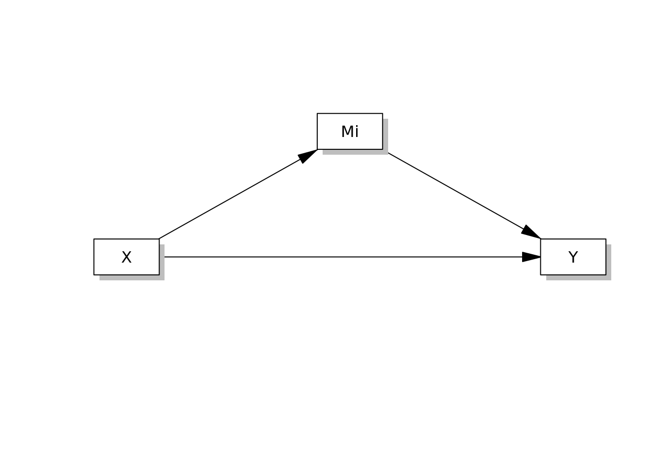
매개효과 분석은 설명변수가 반응변수에 영향을 미치는 경로, 매커니즘을 확인하기 위한 분석방법입니다. 단순매개모형(4번 모델)은 다음과 같은 다이아그램으로 표현할 수 있습니다.
먼저 R에서 process macro를 사용하려면 패키지를 설치하거나 파일을 다운받아야 합니다. 패키지로는 가톨릭대학교 문건웅 교수님이 만든 processR이라는 패키지를 다음과 같이 다운로드하고 불러올 수 있습니다.
devtools::install_github("cardiomoon/processR")
library(processR)
processR 패키지를 사용하려면 lavaan 패키지가 필요합니다. 아래 코드로 다운로드하고 불러올 수 있습니다.
install.packages("lavaan")
library(lavaan)
아래 코드로 processR 패키지에서 지원하는 모델의 번호를 확인할 수 있습니다.
pmacro$no [1] 0.0 1.0 2.0 3.0 4.0 4.2 5.0 6.0 6.3 6.4 7.0 8.0 9.0 10.0 11.0
[16] 12.0 13.0 14.0 15.0 16.0 17.0 18.0 19.0 20.0 21.0 22.0 23.0 24.0 28.0 29.0
[31] 30.0 31.0 35.0 36.0 40.0 41.0 45.0 49.0 50.0 58.0 59.0 60.0 61.0 62.0 63.0
[46] 64.0 65.0 66.0 67.0 74.0 75.0 76.0 25.0 26.0 27.0 58.2 4.3직접 다운받아 사용하시려면 process macro를 개발한 Andrew F. Hayes가 제공하는 파일을 여기서 내려받을 수 있습니다. process.R파일을 실행시키거나 분석을 진행할 R파일 상단에 source("process.R")코드를 실행하면 함수를 사용할 수 있습니다. processR패키지와 process.R파일은 서로 다른 도구이니 혼동하지 않도록 주의해야 합니다. 이 포스트에서 processR 패키지에서 제공하는 함수는 코드 상단에 # processR로, process.R에서 제공하는 함수는 # process.R로 주석을 달아놓겠습니다.
예시 데이터로 단순매개효과를 설명해보겠습니다.
미국의 1,338명의 의료비용에 대한 데이터입니다.
cost <- read.csv("Medical_Cost.csv")| age | sex | bmi | children | smoker | region | charges |
|---|---|---|---|---|---|---|
| 19 | female | 27.900 | 0 | yes | southwest | 16884.924 |
| 18 | male | 33.770 | 1 | no | southeast | 1725.552 |
| 28 | male | 33.000 | 3 | no | southeast | 4449.462 |
| 33 | male | 22.705 | 0 | no | northwest | 21984.471 |
| 32 | male | 28.880 | 0 | no | northwest | 3866.855 |
process.R의 process()함수를 실행해보겠습니다. 인자는 다음과 같습니다.
data = 데이터셋
x = 설명변수
y = 반응변수
m = 매개변수
model = 모델번호
boot = 부트스트래핑 횟수
total = 총효과 출력(0이면 출력하지 않음)
********************* PROCESS for R Version 4.3.1 *********************

           Written by Andrew F. Hayes, Ph.D.  www.afhayes.com
   Documentation available in Hayes (2022). www.guilford.com/p/hayes3

***********************************************************************

Model : 4
    Y : charges
    X : smoker
    M : bmi

Sample size: 1338


***********************************************************************
Outcome Variable: bmi

Model Summary:
          R      R-sq       MSE         F       df1       df2         p
     0.0038    0.0000   37.2152    0.0188    1.0000 1336.0000    0.8910

Model:
             coeff        se         t         p      LLCI      ULCI
constant   30.6518    0.1870  163.8953    0.0000   30.2849   31.0187
smoker      0.0567    0.4133    0.1371    0.8910   -0.7541    0.8674

***********************************************************************
Outcome Variable: charges

Model Summary:
          R      R-sq           MSE         F       df1       df2         p
     0.8111    0.6579 50238769.3992 1283.9234    2.0000 1335.0000    0.0000

Model:
              coeff        se         t         p       LLCI       ULCI
constant -3459.0955  998.2795   -3.4651    0.0005 -5417.4628 -1500.7282
smoker   23593.9810  480.1805   49.1357    0.0000 22651.9905 24535.9715
bmi        388.0152   31.7875   12.2065    0.0000   325.6564   450.3741

************************ TOTAL EFFECT MODEL ***************************
Outcome Variable: charges

Model Summary:
          R      R-sq           MSE         F       df1       df2         p
     0.7873    0.6198 55804130.1996 2177.6149    1.0000 1336.0000    0.0000

Model:
              coeff        se         t         p       LLCI       ULCI
constant  8434.2683  229.0142   36.8286    0.0000  7985.0017  8883.5348
smoker   23615.9635  506.0753   46.6649    0.0000 22623.1748 24608.7523

************ TOTAL, DIRECT, AND INDIRECT EFFECTS OF X ON Y ************

Total effect of X on Y:
      effect        se         t         p       LLCI       ULCI
  23615.9635  506.0753   46.6649    0.0000 22623.1748 24608.7523

Direct effect of X on Y:
      effect        se         t         p       LLCI       ULCI
  23593.9810  480.1805   49.1357    0.0000 22651.9905 24535.9715

Indirect effect(s) of X on Y:
       Effect
bmi   21.9825

******************** ANALYSIS NOTES AND ERRORS ************************

Level of confidence for all confidence intervals in output: 95
우선 Figure.1에서 보았던 경로의 이름을 정하겠습니다.
\(X → M : a\)
\(M → Y : b\)
\(X → Y : c'\)
단순매개모형에서 설명변수가 0, 1로 이루어진 변수일때, \(a = [\bar{M}|(X = 1)] - [\bar{M}|(X = 0)] = 0.0567\)이며 X가 1일때 M의 평균과 X가 0일때 M의 평균의 차이와 같고 lm(bmi ~ smoker, data = cost)의 기울기와 같습니다.
\(b = [\hat{Y}|(M = m, X = x)] - [\hat{Y}|(M = m - 1, X = x)] = 388.0152\)이며 이는 lm(charges ~ smoker + bmi, data = cost)에서 bmi의 기울기와 같고 아래처럼 계산할 수도 있습니다.
       1
388.0152
\(c' = [\hat{Y}|(X = x, M = m)] - [\hat{Y}|(X = x - 1, M = m)] = 23593.9810\)이며 lm(charges ~ smoker + bmi, data = cost)의 smoker의 기울기와 같고 다음과 같이 계산할 수도 있습니다.
       1
23593.98
단순매개모형에서 \(ab\)를 간접효과, \(c'\)을 직접효과, 이 둘을 더한 값을 \(c\)(총효과)라고 하며 총효과는 lm(charges ~ smoker, data = cost)의 기울기와 같습니다.
간접효과는 매개변수를 통했을 때 흡연자는 비흡연자보다 의료비용이 21.9825만큼 높다는 것을 의미하며, 직접효과는 매개변수가 고정되어있을 때 흡연자는 의료비용이 23593.981만큼 더 높다는 것을 의미합니다.
이제 processR 패키지를 실행해보겠습니다.
# processR
labels <- list(X = "smoker", Y = "charges", M = "bmi")
meanSummaryTable(labels = labels, data = cost)
|
Y |
M |
Y |
|
|---|---|---|---|---|
charges |
bmi |
adjusted |
||
smoker(X) = 0 |
Mean |
8434.268 |
30.652 |
8438.77 |
SD |
5993.782 |
6.043 |
||
smoker(X) = 1 |
Mean |
32050.232 |
30.708 |
32032.751 |
SD |
11541.547 |
6.319 |
||
Mean |
13270.422 |
30.663 |
||
SD |
12110.011 |
6.098 |
Adjusted mean은 \(adjusted\;mean(\bar{Y}^*) = i_{Y} + b\bar{M} + c'X\)로 계산할 수 있습니다. 설명변수가 0일때는 \(\bar{Y}^* = -3459.10 + 388.02 * 30.6634 + 23593.98 * 0\)이고 설명변수가 1일때는 \(\bar{Y}^* = -3459.10 + 388.02 * 30.6634 + 23593.98 * 1\)로 계산할 수 있습니다. 보정평균은 \(X\)일때 평균적인 \(M\)의 값을 가지는 사람은 보정평균만큼의 \(Y\)를 갖는다는 것을 의미합니다.
아래처럼 각 계수를 깔끔하게 출력하는 함수도 존재합니다.
# processR
modelsSummaryTable(labels = labels, data = cost)
Consequent |
|||||||||||
|---|---|---|---|---|---|---|---|---|---|---|---|
bmi(M) |
charges(Y) |
||||||||||
Antecedent |
Coef |
SE |
t |
p |
Coef |
SE |
t |
p |
|||
smoker(X) |
a |
0.057 |
0.413 |
0.137 |
.891 |
c' |
23593.981 |
480.180 |
49.136 |
<.001 |
|
bmi(M) |
b |
388.015 |
31.787 |
12.207 |
<.001 |
||||||
Constant |
iM |
30.652 |
0.187 |
163.895 |
<.001 |
iY |
-3459.096 |
998.279 |
-3.465 |
.001 |
|
Observations |
1338 |
1338 |
|||||||||
R2 |
0.000 |
0.658 |
|||||||||
Adjusted R2 |
-0.001 |
0.657 |
|||||||||
Residual SE |
6.100 ( df = 1336) |
7087.931 ( df = 1335) |
|||||||||
F statistic |
F(1,1336) = 0.019, p = .891 |
F(2,1335) = 1283.923, p < .001 |
|||||||||
간접효과, 직접효과, 총효과를 다음 함수로 출력할 수 있습니다.
# processR
model <- tripleEquation(labels = labels)
semfit <- sem(model = model, data = cost)

medSummaryTable(semfit)
Effect |
Equation |
estimate |
95% CI |
|---|---|---|---|
indirect |
(a)*(b) |
21.983 |
(-292.098 to 336.063) |
direct |
c |
23593.981 |
(22653.900 to 24534.062) |
total |
direct+indirect |
23615.964 |
(22624.816 to 24607.111) |
prop.mediated |
indirect/total |
0.001 |
(-0.012 to 0.014) |
조절효과
조절효과는 설명변수가 반응변수에 미치는 영향이 다른 변수에 의해 변화될 때, 이 변화를 조절효과라고 하며, 이러한 영향을 주는 변수를 조절변수라고 합니다.
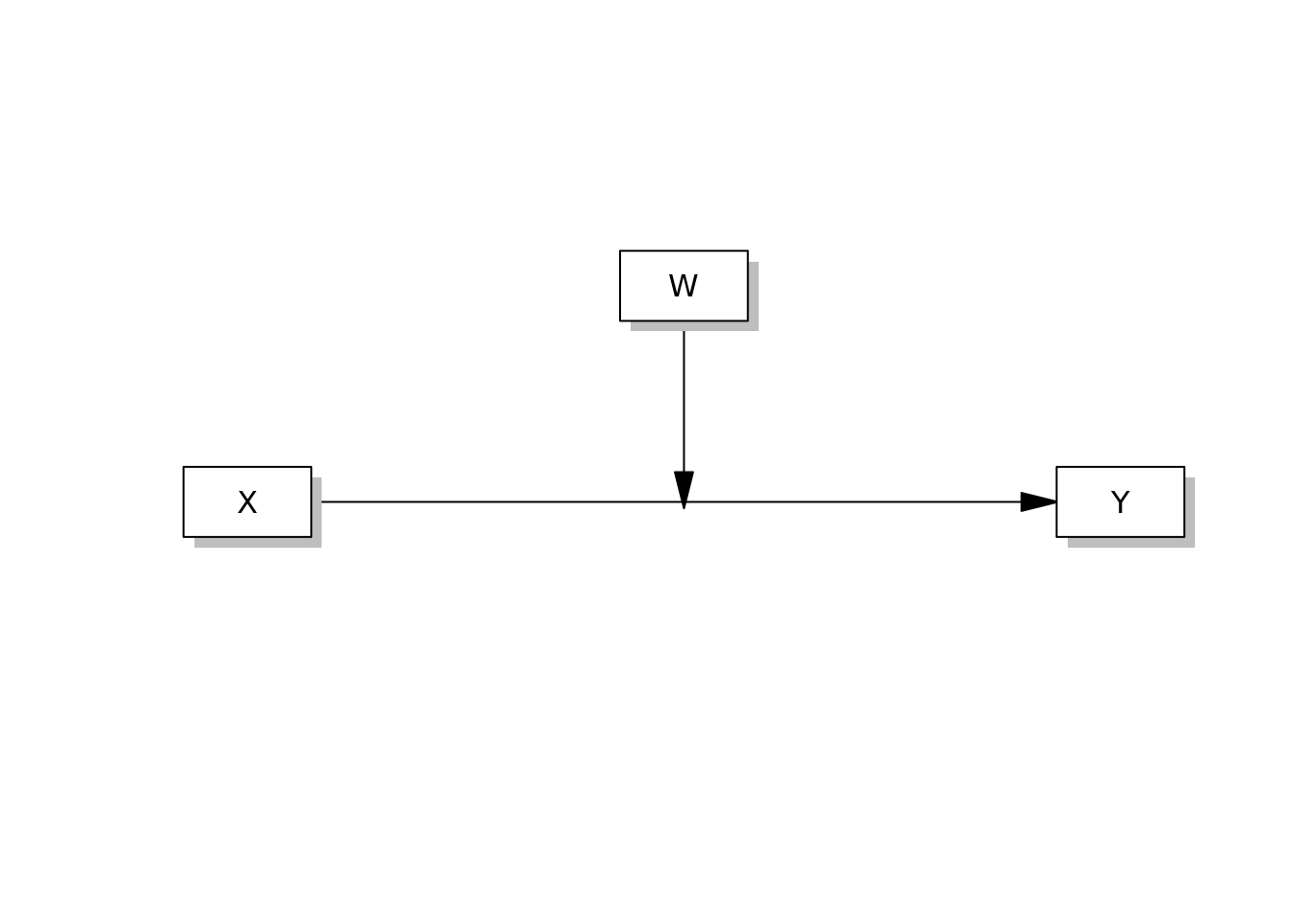
단순조절효과(1번모델)는 다음의 다이아그램으로 나타낼 수 있습니다.
process()함수로 단순조절효과를 알아보겠습니다. plot 인자는 출력결과 하단에 테이블을 만드어줍니다.
# process.R
process(data = cost, x = "smoker", y = "charges", w = "age", model = 1, plot = 1)
********************* PROCESS for R Version 4.3.1 *********************

           Written by Andrew F. Hayes, Ph.D.  www.afhayes.com
   Documentation available in Hayes (2022). www.guilford.com/p/hayes3

***********************************************************************

Model : 1
    Y : charges
    X : smoker
    W : age

Sample size: 1338


***********************************************************************
Outcome Variable: charges

Model Summary:
          R      R-sq           MSE         F       df1       df2         p
     0.8495    0.7217 40903347.7298 1153.1995    3.0000 1334.0000    0.0000

Model:
              coeff        se         t         p       LLCI       ULCI
constant -2091.4206  582.5654   -3.5900    0.0003 -3234.2647  -948.5764
smoker   22385.5487 1278.7311   17.5061    0.0000 19877.0057 24894.0917
age        267.2489   13.9285   19.1872    0.0000   239.9247   294.5731
Int_1       37.9887   31.0950    1.2217    0.2220   -23.0116    98.9890

Product terms key:
Int_1  :  smoker  x  age

Test(s) of highest order unconditional interaction(s):
      R2-chng         F       df1       df2         p
X*W    0.0003    1.4925    1.0000 1334.0000    0.2220
----------
Focal predictor: smoker (X)
      Moderator: age (W)

Data for visualizing the conditional effect of the focal predictor:
     smoker       age    charges
     0.0000   22.0000  3788.0555
     1.0000   22.0000 27009.3554
     0.0000   39.0000  8331.2870
     1.0000   39.0000 32198.3946
     0.0000   56.0000 12874.5186
     1.0000   56.0000 37387.4338

******************** ANALYSIS NOTES AND ERRORS ************************

Level of confidence for all confidence intervals in output: 95
단순조절효과의 계수는 lm(charges ~ smoker + age + smoker * charges, data = cost)의 계수와 동일합니다.
\(\hat{Y} = i_{Y} + b_{1}X + b_{2}W + b_{3}XW\)일때, \(b_{1} = 23385.55\), \(b_{2} = 267.25\), \(b_{3} = 37.99\)이며 각 계수를 다음과 같은 의미를 가지고 있습니다.
\(b_{1} = W\)가 \(0\)일때 \(X\)가 \(Y\)에 미치는 조건부 효과이고 \(X\)가 \(Y\)에 미치는 조건부 효과는 \(\theta_{X→Y} = b_{1} + b_{3}W\)로 계산합니다.
\(b_{2} = X\)가 \(0\)일때 \(W\)가 \(Y\)에 미치는 조건부 효과이고 \(W\)가 \(Y\)에 미치는 조건부 효과는 \(\theta_{W→Y} = b_{2} + b_{3}X\)로 계산합니다.
\(b_{3} = W\)가 한 단위 바뀔 때, \(X\)의 한 단위 변화가 \(Y\)에 영향을 미치는 정도의 차이입니다.
proceeR 패키지로 확인해보겠습니다.
Consequent |
|||||
|---|---|---|---|---|---|
charges(Y) |
|||||
Antecedent |
Coef |
SE |
t |
p |
|
smoker(X) |
c1 |
22385.549 |
1278.731 |
17.506 |
<.001 |
age(W) |
c2 |
267.249 |
13.929 |
19.187 |
<.001 |
smoker:age(X:W) |
c3 |
37.989 |
31.095 |
1.222 |
.222 |
Constant |
iY |
-2091.421 |
582.565 |
-3.590 |
<.001 |
Observations |
1338 |
||||
R2 |
0.722 |
||||
Adjusted R2 |
0.721 |
||||
Residual SE |
6395.573 ( df = 1334) |
||||
F statistic |
F(3,1334) = 1153.199, p < .001 |
||||
마치며
이 포스트에서는 간단한 모델만을 다뤘기 때문에 사용하지 못한 함수나 개념이 많습니다.
추후에 기회가 된다면 포스트를 수정보완하여 좀 더 복잡한 모델을 소개할 수 있기를 바랍니다.
Process macro에 대해 좀 더 알고 싶으신 분들은 문재성 교수님의 processRWorkshop 또는 Andrew F. Hayes의 “Introduction to Mediation, Moderation, and Conditional Process Analysis”를 참고하시면 도움이 될 수 있습니다.
Citation
BibTeX citation:
@online{choi2024,
  author = {Choi, Heeseok},
  title = {Process Macro {소개}},
  date = {2024-03-14},
  url = {https://blog.zarathu.com/posts/2024-03-14-process-macro/},
  langid = {en}
}
For attribution, please cite this work as:
Choi, Heeseok. 2024. “Process Macro 소개.” March 14. https://blog.zarathu.com/posts/2024-03-14-process-macro/.