Data visualization plays an important role in data analysis. Fortunately, R has many advantages over other programming languages, led by ggplot2, in this regard.
On the other hand, data visualization sometimes requires additional custom modifications such as color or layout. Although it would be great if you could do this within R, sometimes it is more convenient to use an external program like ppt for simple tasks than to use multiple lines of code.
In a previous article, I introduced how to create and edit vector images in MS powerpoint using the officer package. In this article, I will introduce advanced methods in R and R packages used to create and edit multiple images.
result
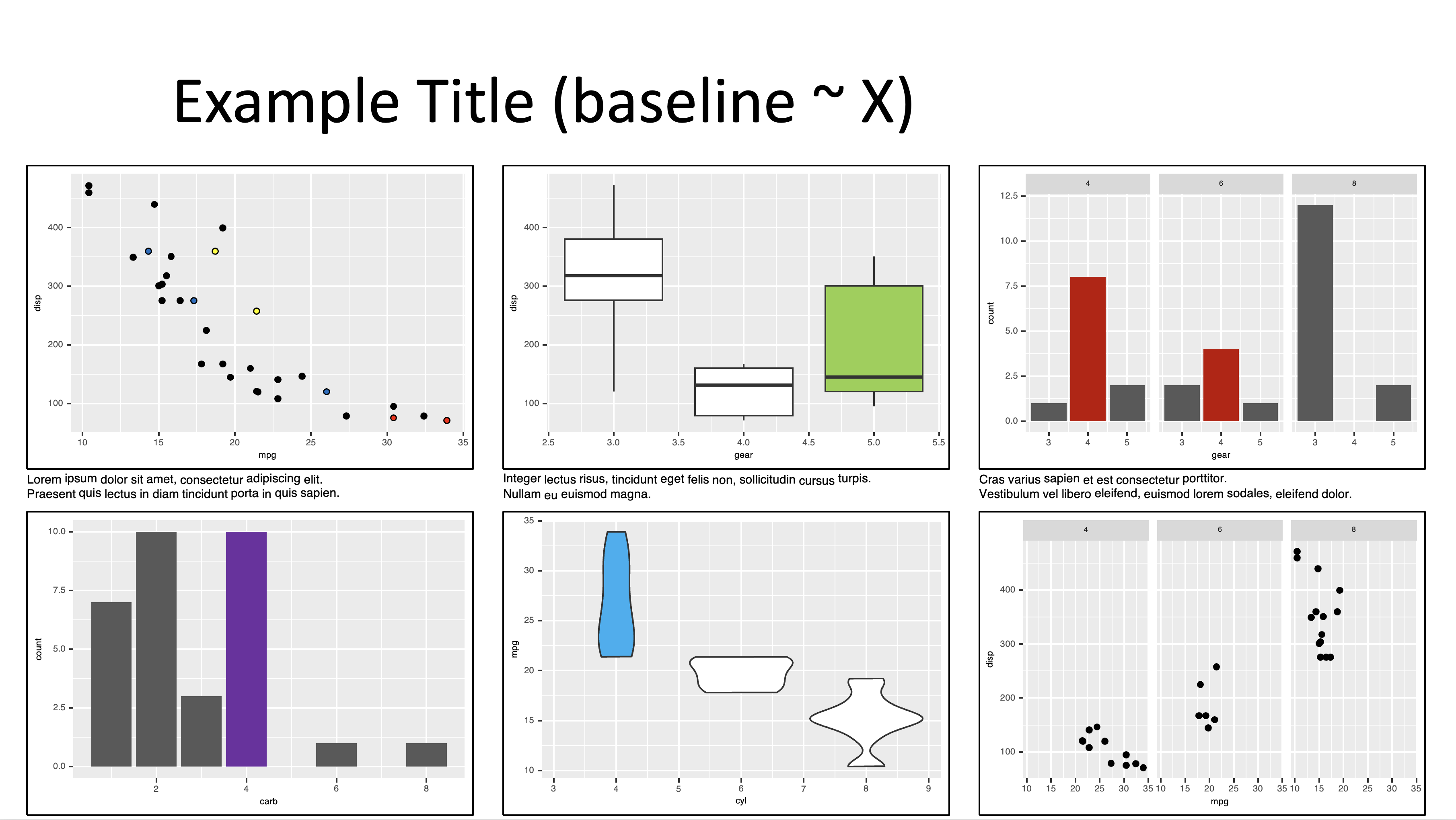
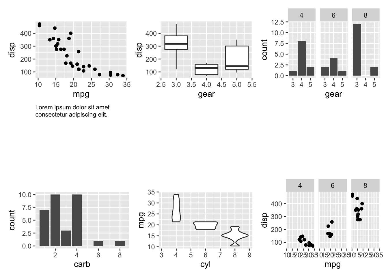
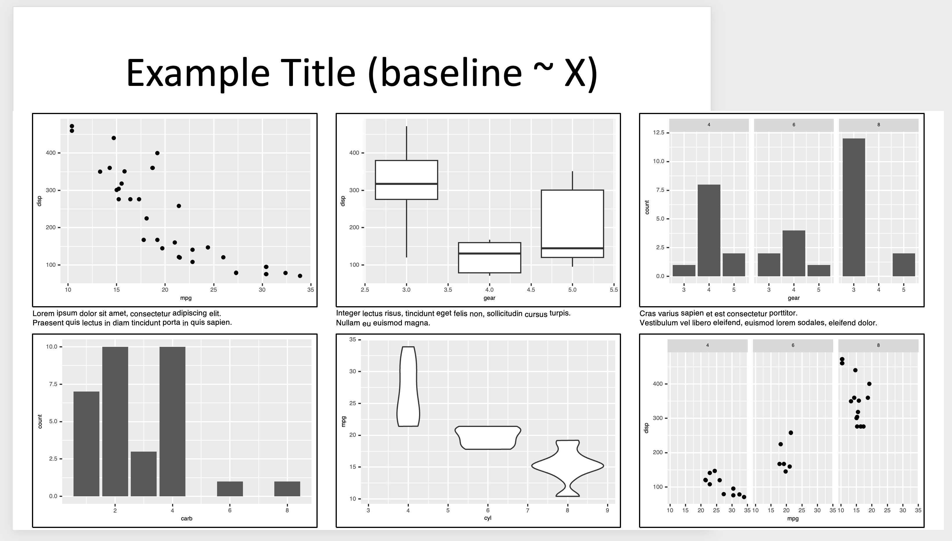
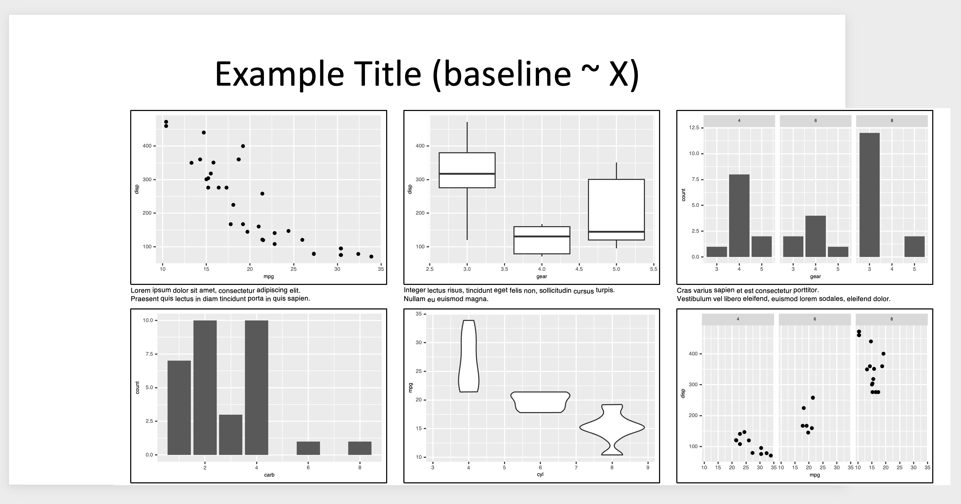
First, let me introduce the ppt results using the methods introduced in this article.
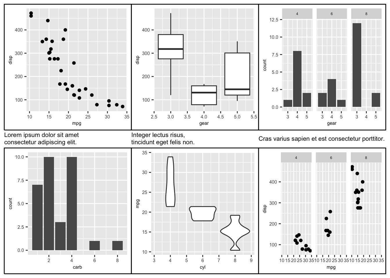
First, the above image is the result of
Visualization created using ggplot2 in R
Wrapped in a box using cowplot
Layout using patchwork to arrange visualization and text for explanation
Created in MS powerpoint with wide screen (or 16:9) resolution using officer.
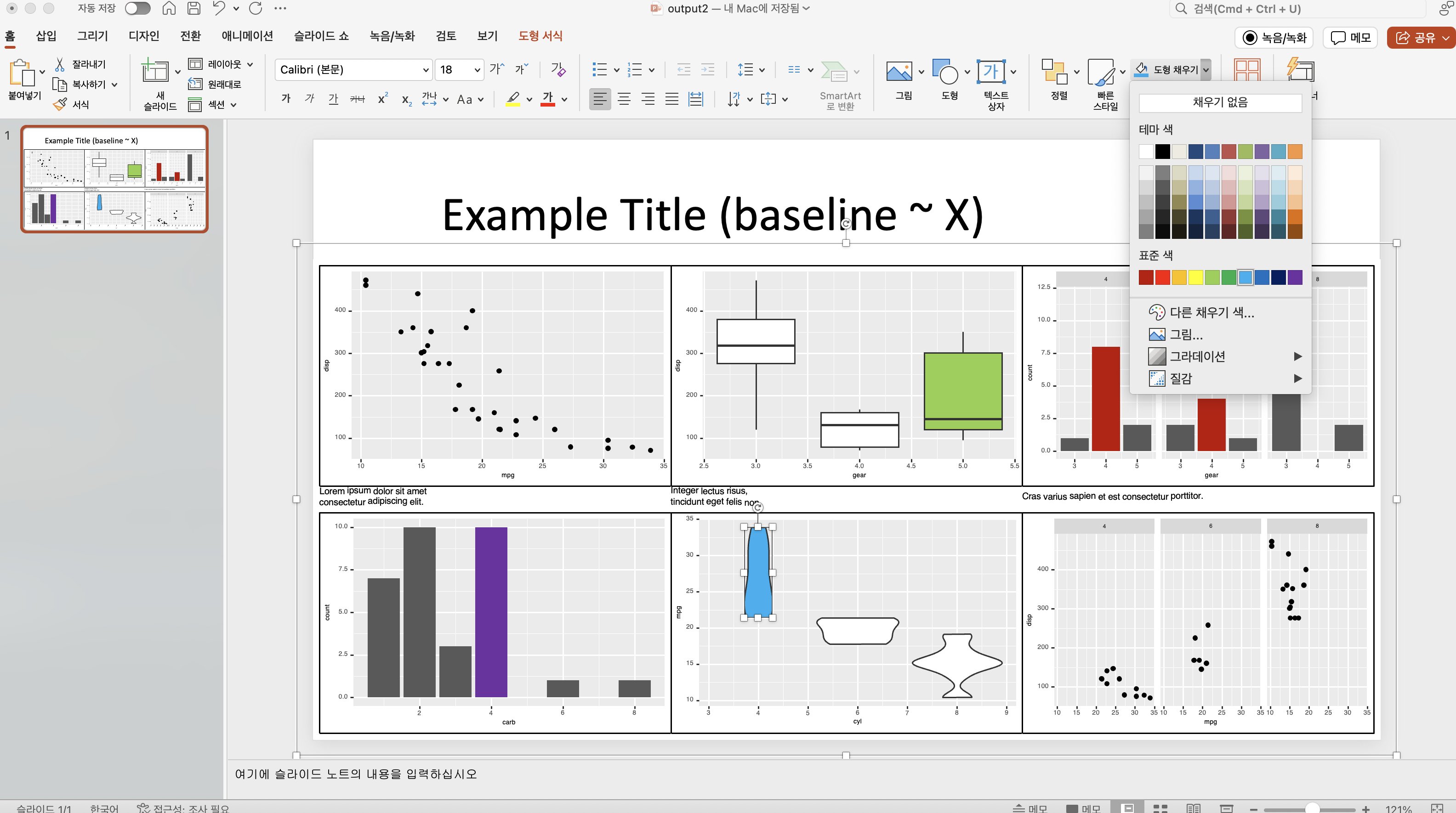
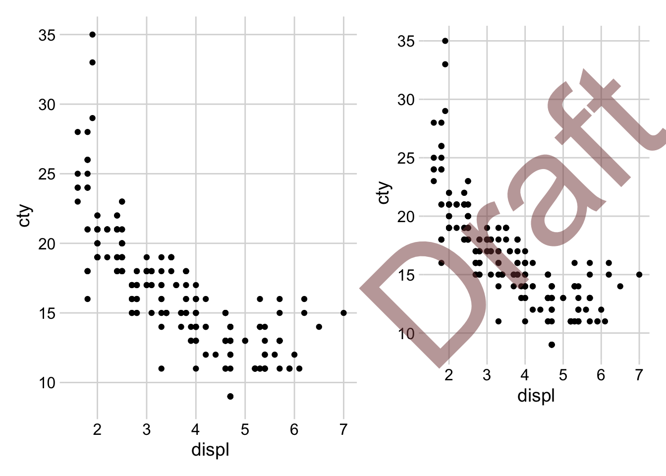
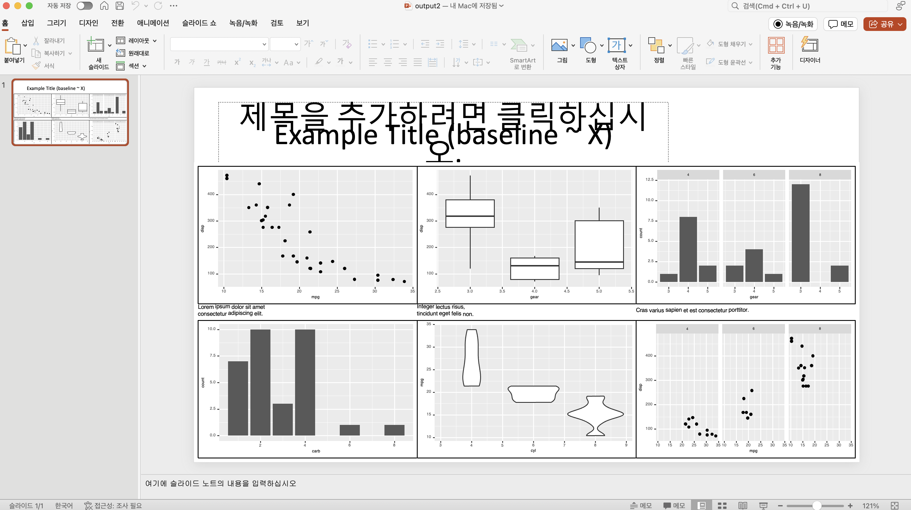
Since these results use vector graphics, they can be easily customized in ppt as shown in the following image.
patchwork
The example images used in this article are based on the example code of patchwork using the mtcars dataset of ggplot2. I will not explain ggplot2 and each chart separately.
mpg
cyl
disp
hp
drat
wt
qsec
vs
am
gear
carb
Mazda RX4
21.0
6
160.0
110
3.90
2.620
16.46
0
1
4
4
Mazda RX4 Wag
21.0
6
160.0
110
3.90
2.875
17.02
0
1
4
4
Datsun 710
22.8
4
108.0
93
3.85
2.320
18.61
1
1
4
1
Hornet 4 Drive
21.4
6
258.0
110
3.08
3.215
19.44
1
0
3
1
Hornet Sportabout
18.7
8
360.0
175
3.15
3.440
17.02
0
0
3
2
Valiant
18.1
6
225.0
105
2.76
3.460
20.22
1
0
3
1
Duster 360
14.3
8
360.0
245
3.21
3.570
15.84
0
0
3
4
Merc 240D
24.4
4
146.7
62
3.69
3.190
20.00
1
0
4
2
Merc 230
22.8
4
140.8
95
3.92
3.150
22.90
1
0
4
2
Merc 280
19.2
6
167.6
123
3.92
3.440
18.30
1
0
4
4
Merc 280C
17.8
6
167.6
123
3.92
3.440
18.90
1
0
4
4
Merc 450SE
16.4
8
275.8
180
3.07
4.070
17.40
0
0
3
3
Merc 450SL
17.3
8
275.8
180
3.07
3.730
17.60
0
0
3
3
Merc 450SLC
15.2
8
275.8
180
3.07
3.780
18.00
0
0
3
3
Cadillac Fleetwood
10.4
8
472.0
205
2.93
5.250
17.98
0
0
3
4
Lincoln Continental
10.4
8
460.0
215
3.00
5.424
17.82
0
0
3
4
Chrysler Imperial
14.7
8
440.0
230
3.23
5.345
17.42
0
0
3
4
Fiat 128
32.4
4
78.7
66
4.08
2.200
19.47
1
1
4
1
Honda Civic
30.4
4
75.7
52
4.93
1.615
18.52
1
1
4
2
Toyota Corolla
33.9
4
71.1
65
4.22
1.835
19.90
1
1
4
1
Toyota Corona
21.5
4
120.1
97
3.70
2.465
20.01
1
0
3
1
Dodge Challenger
15.5
8
318.0
150
2.76
3.520
16.87
0
0
3
2
AMC Javelin
15.2
8
304.0
150
3.15
3.435
17.30
0
0
3
2
Camaro Z28
13.3
8
350.0
245
3.73
3.840
15.41
0
0
3
4
Pontiac Firebird
19.2
8
400.0
175
3.08
3.845
17.05
0
0
3
2
Fiat X1-9
27.3
4
79.0
66
4.08
1.935
18.90
1
1
4
1
Porsche 914-2
26.0
4
120.3
91
4.43
2.140
16.70
0
1
5
2
Lotus Europa
30.4
4
95.1
113
3.77
1.513
16.90
1
1
5
2
Ford Pantera L
15.8
8
351.0
264
4.22
3.170
14.50
0
1
5
4
Ferrari Dino
19.7
6
145.0
175
3.62
2.770
15.50
0
1
5
6
Maserati Bora
15.0
8
301.0
335
3.54
3.570
14.60
0
1
5
8
Volvo 142E
21.4
4
121.0
109
4.11
2.780
18.60
1
1
4
2
mtcars
library(ggplot2)p1<-ggplot(mtcars)+geom_point(aes(mpg, disp))p2<-ggplot(mtcars)+geom_boxplot(aes(gear, disp, group =gear))p3<-ggplot(mtcars)+geom_bar(aes(gear))+facet_wrap(~cyl)p4<-ggplot(mtcars)+geom_bar(aes(carb))p5<-ggplot(mtcars)+geom_violin(aes(cyl, mpg, group =cyl))p6<-ggplot(mtcars)+geom_point(aes(mpg, disp))+facet_wrap(~cyl)
patchwork is an R package that allows you to easily arrange multiple ggplot results on one (page) graphic. For similar purposes, other packages such as gridExtra or cowplot can also be used.
The usage of patchwork consists of +, |, ( ), and /.
| (vertical bar)
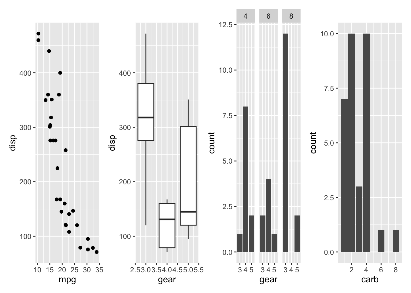
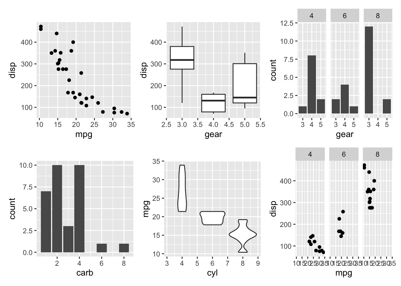
First, | is used to arrange multiple images in one row.
p1|p2|p3|p4
patchwork - vertical bar
+
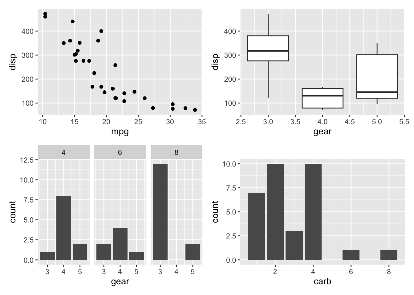
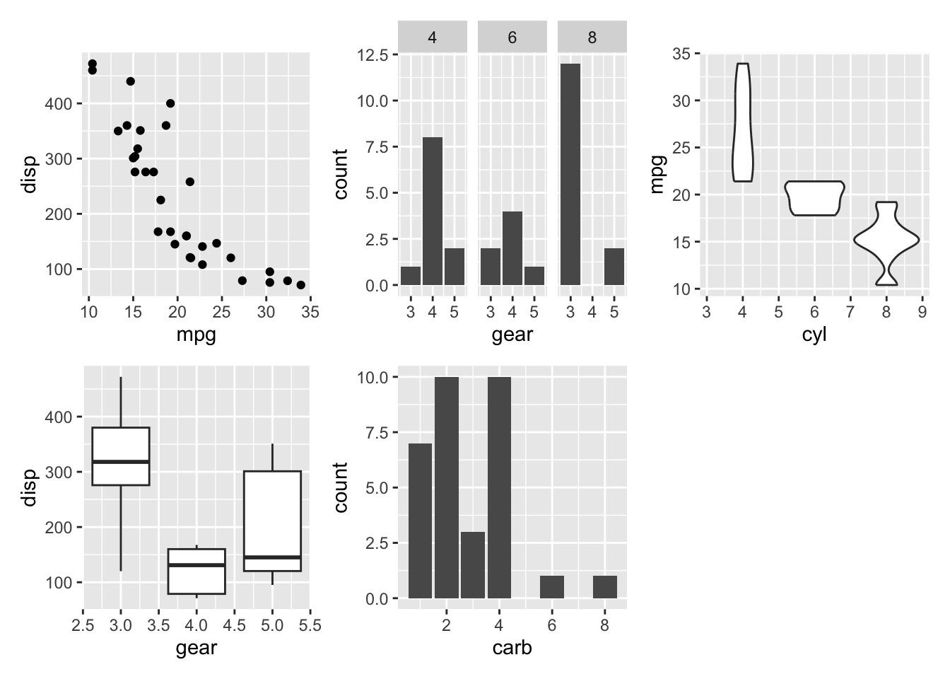
Second, + is used to arrange multiple images, filling the rows and columns in grid form, in row order.
p1+p2+p3+p4
patchwork - plus
To specify the image layout, use the plot_layout function
p1+p2+p3+p4+p5+plot_layout(ncol =3, byrow =FALSE)
patchwork - plot_layout
/
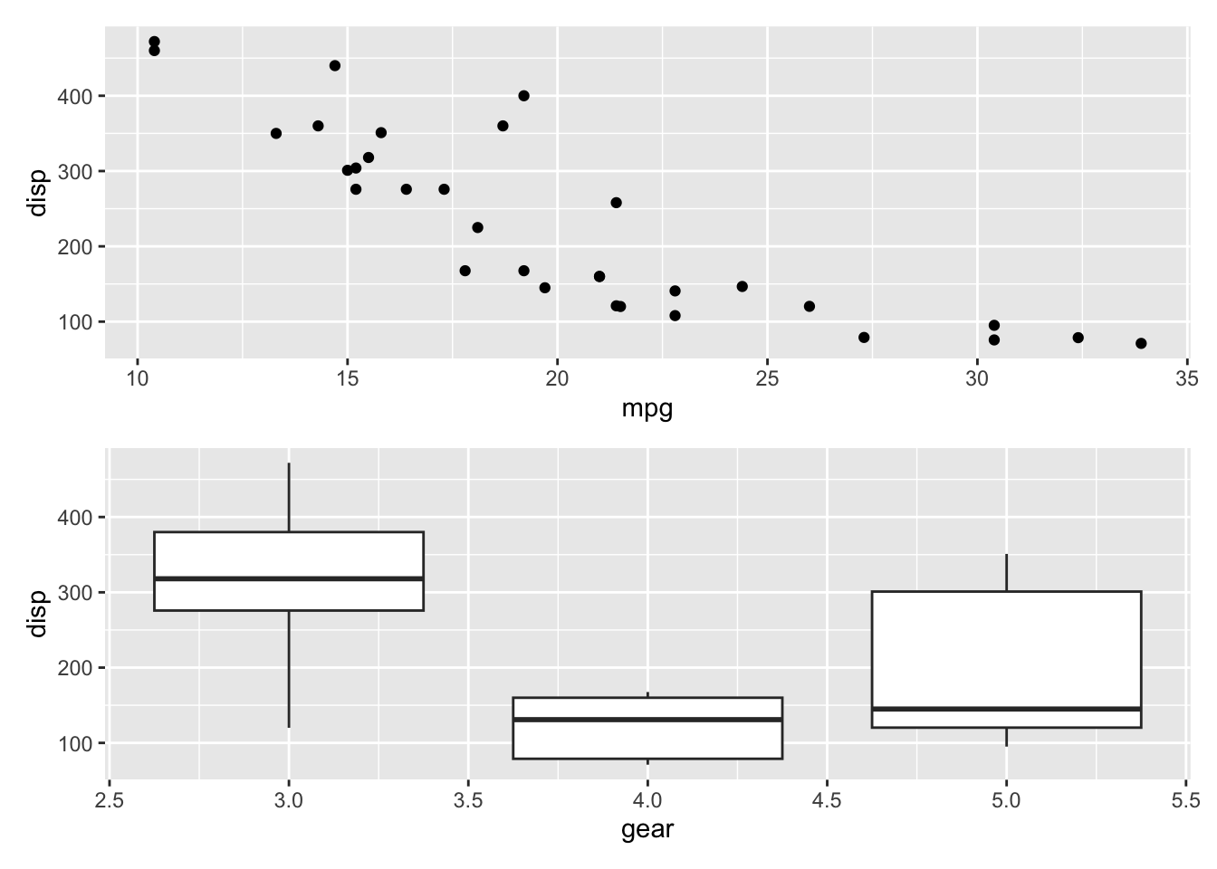
Next, using / allows you to arrange images vertically
p1/p2
patchwork - slash
( )
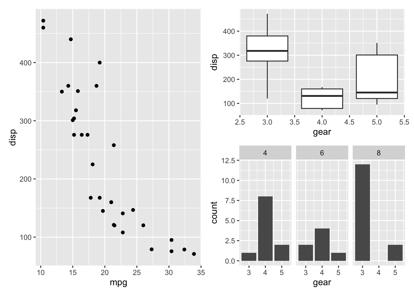
Finally, using ( ) allows you to group images into one group
p1|(p2/p3)
patchwork - parenthesis
Of course, patchwork provides various functions. For more information, refer to the official documentation.
Now, let’s use this to arrange the 6 example images we created earlier on one page of a ppt.
However, in this state, an error occurs because the text object contains only simple text, not ggplot results. To resolve this, use the ggdraw function in cowplot.
ggdraw
First, cowplot is an R package that provides functions to add annotations and themes to ggplot2 results. Think of ggdraw as adding a top-level layer to ggplot2 results so that you can draw additional graphics
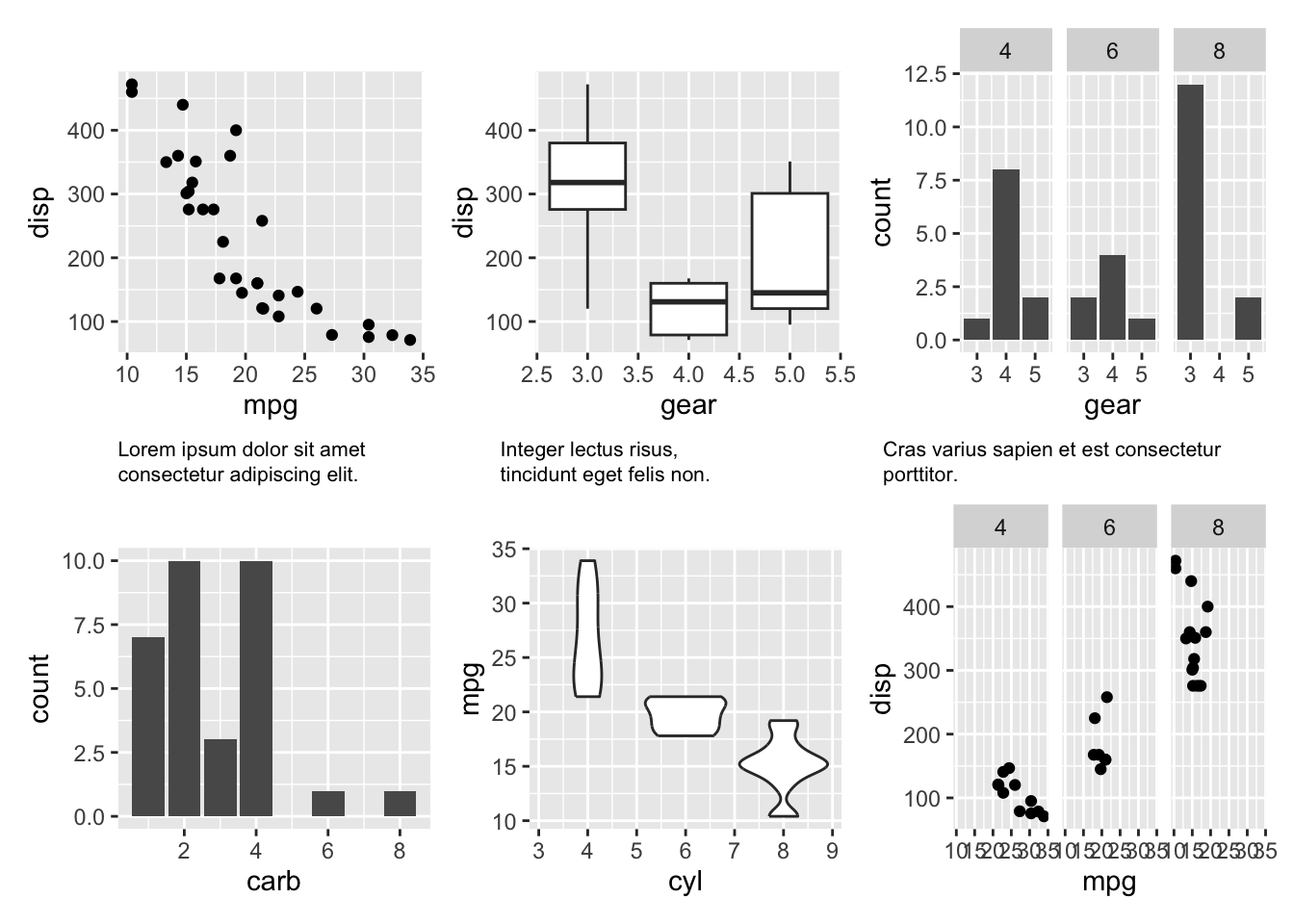
Next, let’s create a separate function for the features that are repeatedly used in customizing labels before adding the remaining labels. In addition, to reduce the caption part, adjust the height using height of plot_layout instead of assigning the same height to the caption and graph in a 1:1:1 ratio.
cowplot - caption function
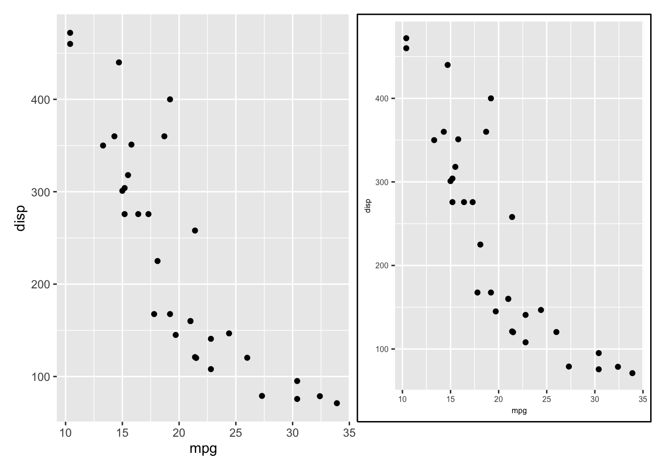
Next, we will cover how to wrap each visualization in a box (border). To do this, we use ggdraw to create a layer for each visualization and use the draw_line function to add a line passing through (0,0) to (1,1) to that layer.
In addition, we use the theme function to adjust the text properties for each visualization
If you don’t use the remove_slide function in the above code, a slide containing the ggplot result will be created after the existing template slide, so you will start with an unnecessary first page as shown below.
On the other hand, if you remove both remove_slide and add_slide and only add an image with ph_with, the title of the template and the newly added title will overlap as shown below.
read_pptx("~/Documents/template.pptx")|>ph_with( value ="Example Title (baseline ~ X)", location =ph_location_type(type ="title"))|>ph_with(rvg::dml(ggobj =combined_plot), location =ph_location(left =0, top =1.5, height =6, width =13.333))|>print(target ="output2.pptx")
Therefore, it is recommended to use remove_slide and add_slide when using a template.
summary
In this article, we learned how to combine multiple graphs using patchwork and cowplot, make slight customizations, and add them to a ppt using officer. There are various ways to connect R’s functions with ppt, and through this, you will be able to work more efficiently.
The final code is as follows.
This content is translated with github copilot
Code
library(ggplot2)library(patchwork)library(cowplot)library(officer)p1<-ggplot(mtcars)+geom_point(aes(mpg, disp))p2<-ggplot(mtcars)+geom_boxplot(aes(gear, disp, group =gear))p3<-ggplot(mtcars)+geom_bar(aes(gear))+facet_wrap(~cyl)p4<-ggplot(mtcars)+geom_bar(aes(carb))p5<-ggplot(mtcars)+geom_violin(aes(cyl, mpg, group =cyl))p6<-ggplot(mtcars)+geom_point(aes(mpg, disp))+facet_wrap(~cyl)text<-list( p1 ="Lorem ipsum dolor sit amet <br> consectetur adipiscing elit.", p2 ="Integer lectus risus, <br> tincidunt eget felis non.", p3 ="Cras varius sapien et est consectetur porttitor.")cap<-function(text){ggdraw()+labs(subtitle =text)+theme_void()+theme( text =element_text(size =8), plot.margin =margin(0, 0, 0, 0))}text_theme<-theme( text =element_text(size =6), axis.text =element_text(size =6), axis.title =element_text(size =6), axis.title.x =element_text(size =6), axis.title.y =element_text(size =6), plot.title =element_text(size =6), legend.text =element_text(size =6), legend.title =element_text(size =6))with.box<-function(p){ggdraw(p+text_theme)+cowplot::draw_line( x =c(0, 1, 1, 0, 0), y =c(0, 0, 1, 1, 0), color ="black", size =0.5)}combined_plot<-(with.box(p1)|with.box(p2)|with.box(p3))/(cap(text$p1+text_theme)|cap(text$p2+text_theme)|cap(text$p3+text_theme))/(with.box(p4)|with.box(p5)|with.box(p6))+plot_layout(heights =c(5, 0.1, 5))+theme(plot.margin =margin(1, 10, 1, 10))combined_plotread_pptx("~/Documents/template.pptx")|>ph_with( value ="Example Title (baseline ~ X)", location =ph_location_type(type ="title"))|>ph_with(rvg::dml(ggobj =combined_plot), location =ph_location(left =0, top =1.5, height =6, width =13.333))|>print(target ="output2.pptx")